N e w t o n I n t e r p o l a t i o n P o l y n o m i a l : P r o j e c t NIP_1
-
Given the following n+1 (measurements) points
Table: Values (Xi,Yi) i=0,n; Xi≠Xk ∀i≠kNo. 0 1 2 ... i ... n X-value X0 X1 X2 ... Xi ... Xn Y-value Y0 Y1 Y2 ... Yi ... Yn All (X,Y) values are supposed connected according to (unknown) function y=f(x), of which only a few value pairs have been collected (measured). An example of such measurement could be the resistivity of a metal (R=y-values) in function of its temperature (T=x-values). Electrical resistivity usually increases with temperature according to following relationship: R(T) = c0 + c1.T + c2 T2.
A general objective is to express functional relationships y=F(x) from the set of known values {(Xi,Yi)}, with F; F(x)≈f(x) ∀x. There are many methods to define F. The Newton Interpolation Polynomial method (NIP) is based on following assumptions:
NIP is an interpolation method
eq. [1] F(xi)=yi, ∀i, i=0,n -
F(x) is a polynomial
eq. [2] F(x) = c0 + c1.x + ... + ci.xi + .. + cn.xn - ci, i=0,n called the polynomial coefficients are constants ∈ ℝ (real numbers) or more generally ∈ ℂ (complex numbers),
- xi, i=0,n are powers of x, which define the polynomial basis
eq. [2] writes F(x) in canonical form. Newton and Lagrange resolve the interpolation by transposing F(x) into non-canonical equivalents.
-
Newton rewrites F(x) as follows:
eq. [3] F(x)=N(x)=Nn(x)= y0 + b1(x-x0) + ... + bi(x-x0)(x-x1)...(x-xi-1) + ... + bn(x-x0)...(x-xn-1) Nn(x) is the Newton Interpolation Polynomial of degree n associated with the n+1 measures (xi,yi), i=0,n.
The followings results of Numerical Analysis may help better understand the mathematics behind NIP.
-
Fundamental theorem of algebra
Every non-constant single-variable polynomial with complex coefficients has at least one complex root.
witheq. [4] Pn(X) = c0 + c1.X + ... + ci.Xi + .. + cn.Xn = 0
- i=0,n ∈ℕ
- Xi is the power i of complex variable X
- ci are constant coefficients ∈ ℂ (the field of complex numbers)
eq. [4] has at least one solution, X0 (= root of the equation).
Following consequences are derived from the fundamental theorem of algebra (or can be considered as alternative formulations):
-
(Through the use of successive polynomial division)
In the field of complex numbers eq. [4] has exactly n roots Xi, i=1,n , each counted with its multiplicity.
-
Be Pn(X) and Qn(X) 2 polynomials on the complex field of degree n.
If both polynomials yield an equal output for at least n+1 values i.e. Pn(xi) = Qn(xi), for xi, i=0,n, and xi ≠ xj for i ≠ j
then Pn(X) = Qn(X) i.e. both polynomials are the same i.e. are defined by the same coefficients.
-
The
 Taylor series
of a real or complex-valued function f(x) that is infinitely differentiable at a real or complex number a is the power series
Taylor series
of a real or complex-valued function f(x) that is infinitely differentiable at a real or complex number a is the power series
Is the complex or real number a equal to 0, the following polynomial development of f(x) is obtainedeq. [5-a] f(x) = f(a) + (f'(a) ⁄ 1!) . (x-a) + ... + (fk(a) ⁄ k!) . (x-a)k + ...
eq. [5-b] f(x) = ∑k=0,∞ (fk(a) ⁄ k!) . (x-a)k
eq. [5-c] f(x) = ∑k=0,∞ (fk(0) ⁄ k!) . xk
In words, if a (infinitely differentiable) function f(x) is exactly known at one point of its definition domain, then it is known everywhere - and can be expressed as a polynomial, whatever precision is initially targeted .
-
Beside Newton, Lagrange proposed another solution, the Lagrange Interpolation Polynomial (LIP)
eq. [6-a] L(x) = ∑k=0,n yk.Lk(x) A solution is obviously found, if Lk satisfy following equations:
eq. [6-b] Lk(xk) = 1 eq. [6-c] Lk(xi) = 0, for i≠k Lagrange proposes to write:
eq. [6-d] Lk(x) = lk.(x-x0)...(x-xk-1).(x-xk+1).(x-xn) eq. [6-e] lk(x) = 1 ⁄ (xk-x0)...(xk-xk-1).(xk-xk+1).(xk-xn ) According to the fundamental theorem of algebra N(x) and L(x) of degree n, interpolating the same set (xi,yi), i=0,n are identical.
The interpolation problem in canonical form reads as a set of inhomogeneous linear equations
Transposed in the matrix formalism:eq. [7-a] Pn(xi) = ∑k=0,n xik . ck = yi eq. [7-b] [A(i,j)].[C(j)] = [Y(i)] a(i,j) = xij x-coordinates of the measurement points cj polynomial coefficients to calculate yj y-coordinates of the measurement points Equations system eq. [7] has a particular form. Its determinant det[A], called 'VanDerMond' determinant, equals to ∏i>j (xi - xj): There is only a solution, if xi≠xk for i≠k. Also the distance between all (xi-xj) should be comparable, to avoid numeric uncertainties.
Neither N(x) nor L(x) is expressed in canonic form ∑k=0,n ck.xk.
The advantage? Avoid resolving the linear equations system in the general form (eq. [7]). This was particularly interesting in former times, as computer did not exist - and even now, if programmers don't dispose of libraries to solve (linear) equations systems in their general form.-
Transposed into the Lagrange basis, the general equations system (eq. [7]) simplifies radically: only the first diagonal remains (each lk coefficient (eq. [6-e]) is calculated directly and independently from each other).
Since the lk coefficients only depend on xk, they can be reused, if measures apply on the same x-values.
A major drawback is that each Lagrange basis function Lk(x) is a polynomial of degree n. Should the number of measurement points change, all basis functions must be re-calculated. Besides the explanatory potential is rather poor. -
Transposed into the Newton basis (eq. [3]), the general equations system (eq. [7]) transcribes into a lower triangular matrix. A way to proceed is to calculate the
divided differences.
In this case, N(x) can be reformulated as follows:
witheq. [8] N(x) = [y0] + [y0,y1](x-x0) +...+ [y0...yi](x-x0)(x-x1)...(x-xi-1) +...+ [y0...yn](x-x0)...(x-xn-1) [y0] = y0 = b0 [y0y1] = ([y1] - [y0]) ⁄ (x1 - x0) = (y1 - y0) ⁄ (x1 - x0) = b1 [y0...yi+1] = ([y1...yi+1] - [y0...yi]) ⁄ (xi+1 - x0) = bi+1 If all x-values are equidistant, simplifications occur:
(xi+1-xi) = constant=h, ∀i=0,n-1 (xi-x0) = i.h x = x0 + h.t, t ∈[0,n] (x in the domain of interpolation) eq. [9] x-xi = h.(t-i), t ∈[0,n] (x in the domain of interpolation) Consequently, the Newton Interpolation Polynomial can be rewritten as follows:
eq. [10-a] N(x) = y0 + Δy0.t + ... + (Δky0 ⁄ k!) . hk .t(t-1)...(t-(k-1)) +... eq. [10-b] N(x) = ∑k=0,n (Δky0 ⁄ k!) . hk .t(t-1)...(t-(k-1)) eq. [10-c] N(x) = ∑k=0,n Δky0 . hk . (t(t-1)...(t-(k-1)) ⁄ k!) eq. [11-a] Δ0y0 =y0 eq. [11-b] Δk+1y0 = (Δky1 - Δky0) It is interesting to note the formal similarity between eq. [10-b] (the Newton development) and eq. [5-b] (the Taylor development).
In fact, the Newton approximation may be considered some sort of discrete Taylor development: The previously calculated coefficients keep their value, as the number of base functions increases i.e. the number of measurement points increases.
-
Before going into details, a few tips about perl that proved helpful.
Table: perl tips used in this projectCommand OptionsThere is a wide range of options that can be used to order to control perl at invocation. My favorites are following:
perl -c NameOfPerlScript
perl will check the syntax of perl script named NameOfPerlScript without executing the program. Beware, a successful check of syntax does not guarantee a successful run.
LiteralsSpecial literals have a dedicated meaning
- __END__ Legal end of code before the actual EOF
- __FILE__ filename
- __LINE__ line number
- __PACKAGE__ package name
Named Code BlocksA total of 5 code blocks are - if present - executed at the beginning or at the end of a running perl program.
-
BEGIN{}
is executed as soon as possible, that is the moment it is completely defined, even the rest of the containing file is parsed. -
END{}
is executed as late as possible, after perl has finished running the program and just before the interpreter is being exited.
-
This perl implementation of the NIP (project NIP_1) is merely an exercise: The way is as important as the objective. For this reason I will briefly mention my Programing Guidelines. The topic is controversial, if treated out of context: Criteria for code evaluation are too manifold and partially contradict one another. Therefore, each company, project, programmer must define their priorities - given the circumstances. And so do I.
In project NIP_1 the priority is code readability - basing on following pillars:
Modularity of code
As far as reasonable, the code will be broken down into (handy) functions (the unitary modules). Functions themselves will be grouped according to their purpose into different 'libraries' (that may be separately stored into different files).Self explaining code
Especially the naming of entities (variables, routines) should be meaningful.Comments
Comments should add value to the bare code. Is the syntax easy to understand, no need for extensive comments.
Is the syntax ambiguous or complex, comments help the readers understand what has been written and why.
Also comments should disclose critical informations that cannot otherwise be expressed into code, e.g. general concept, boundary conditions, scheduling, authors, references.
Some other implementation criteria were ignored:
Minimize code (Laconism)
perl has been known to allow extreme code concision: one line of code can amount to an entire subroutine.
Since the amount of information required to perform a treatment is basically determined by its nature, extreme concision relies on implicit assumptions. Sometimes extremely short code is only made possible because of bugs or non specified features within the environment providing resources (cf. hacks).Minimize resource allocation
Available resources determine duration and limit the (transient) storage required.
-
The NIP resolution discussed here (called NIP_1) is coded into three files:
NIP.pl stores only the main program (that is not labeled as such in the PL file)
It consists almost exclusively in (library) subroutine calls.NIP_Lib.pm stores all NIP-specific subroutines, functions.
Because their number is limited, one single PM file suffices.NIP_input.txt is the input file.
Its name can be re-defined in the command line (CL).
Table: General program structureNIP.pl main program
It consists in following structuring subroutines (in order of invocation):
-
NIP_lib::read_CL_Options
parses the command line that may include following options (in any order).-if AlternativeInputFileName
By default NIP.pl reads NIP_input.txt.-of AlternativeOutputFileName
By default NIP.pl writes NIP_output.txt.-mf AlternativeMessageFileName
By default NIP.pl writes NIP_messages.txt.-v(erbose)
Extensive messages are output (into the messages file).
By default, the verbose mode is deactivated.-d(ebug)
Generates even more messages than the verbose mode.
By default, deactivated.
NIP_lib::read_Section_INPUT_DATA
parses section INPUT_DATA of the input file, describing the NIP problem.Beware: NIP.pl assumes that all xi-values are equidistant. Users need only enter x0 and Delta-x=(xi+1-xi) to define the set of measurement values.
NIP_lib::solve_NIP
evaluates all bi coefficients, i=0,n (n=number of measures - 1) (see eq. [3]).-
NIP_lib::read_Section_ANALYSIS
parses section ANALYSIS of the input file, describing how to assess the calculated NIP.Beware: To define the set of interpolated points, the same method applies as for the measurements set: Users need only enter x0 and Delta-x=(xi+1-xi).
-
NIP_lib::calc_Ys_NIP
calculates an entire set of values (x,y) according to formula:
Nk(x)= ∑i=0,k (bi.∏j=0,i-1 (x-xj)) with k≤n (n= number of interpolation points - 1).If k=n, Nk(x)=N(x) is the complete NIP. Otherwise, it is a partial NIP. (It is interesting to observe how partial NIPs converge into the complete one, when k→n.)
Beware: Values y=N(x) are calculated with
Horner's method.
NIP_lib.pm perl package (PM module),
containing all NIP-specific subroutines mentioned above (and a few more).NIP_input.txt Input file
containing two sections: INPUT_DATA, ANALYSIS.NIP_input.txt is the file name by default.
The user determines a specific name using CL option -if SpecificFileName.txt (for Input File).The program produces following output.
Table: Output files of NIP.plNIP_output.txt This is the main output:
- Displays input data from Section INPUT_DATA that actually impacts onto the resolution.
-
Displays the bi-values
(characterizing the NIP) in format %6.20f
i.e. 20 decimal places!
(It allows to get a rough idea of the numeric precision in the results.) - Displays interpolated (and extrapolated) (xi,yi)-values as determined in Section ANALYSIS, in format %6.9f i.e. 9 decimal places (expected precision of the calculation).
NIP_output.txt is the file name by default.
The user determines a specific name using CL option -of SpecificFileName.txt (for Output File).NIP_messages.txt Displays warnings and errors, depending on parameters debug (mode), verbosity.
The debug mode is set by CL option -d(ebug).
I activated the option to extensively check what the program reads and how.CL option -v(erbose) also increases the amount of messages - less than the debug mode though.
NIP_messages.txt is the file name by default.
The user determines a specific name using CL option -mf SpecificFileName.txt (for Message File).Beware: Results and messages are always displayed onto screen (i.e. standard output). Users only need files, if they want to store results or further process them.
The program is invoked as follows:
Minimum syntax: perl NIP.pl
Maximum syntax: perl NIP.pl -if InputFN.txt -of OutputFN.txt -mf MessageFN.txt -v(erbose) -debug -
Solving the NIP problem means calculating the bi coefficients, as formulated in eq. [3].
eq. [8] or eq. [10] evaluate the b-coefficient of the NIP in general or in case that all xi, i=0,n=number of measures - 1, are equidistant.
Both equations are valuable from an epistemological point of view - help better understand implications of the NIP formulation. They may also be coded intospreadsheet applications
- like Microsoft EXCEL or
LibreOffice calc.
However, I would not recommend such a method.
The perl implementation discussed here directly resorts to the fact that matrix A(i,j) in equations system associated to the NIP (eq. [3]) is lower triangular: bi can be directly calculated, provided that all bk, k=0,i-1 are known. No need for dedicated subroutines operating on matrices. More precisely perl function NIP_lib::solve_NIP relies on following equations:
eq. [12-a] N0(x) = b0 = y0 eq. [12-b] bi = (yi - Ni-1(xi)) / ( xi-x0)...(xi-xi-1), ∀ i=1,n Numerical imprecision will grow as more coefficients must be calculated - at least because of following (interrelated) reasons :
- Values in matrix A(i,j) from equations system in eq. [3] grow increasingly heterogeneous: The matrix becomes worse and worse conditioned.
- In most cases, values of higher bi-coefficients become increasingly tiny and will soon disappear into the numerical noise.
-
Imprecisions in bi values are amplified
into the calculation of subsequent bk, k>i.
This phenomenon applies specifically to NIP.pl and may greatly reduce the number of coefficients correctly estimated.
Above a limit to be determined, I recommend to solve the canonical equations system (eq. [7]), and use algorithms that calculate all bi with the same degree of precision - which includes a preliminary matrix conditioning.
-
- To show how NIP.pl calculates.
- To assess validity and precision of results.
- To show how the Newton Interpolation Polynomial converges in selected cases: Nk(x) -> f(x), k → ∞.
The trick consists in defining a f(x) function in advance and then compare true and interpolated values. Following cases will be analyzed:
Table: Study cases overviewCase Name Definition of f(x) (to be interpolated) List of TXT-files associated to NIP.pl
Case 1: polynomial f1(x)=(1 + x + 0.5 x2 + 0.25 x3 + 2 x5) NIP_input_StudyCase_1_Polynomial.txt
NIP_output_StudyCase_1_Polynomial.txt
NIP_message_StudyCase_1_Polynomial.txt
Case 2: exponential function f2(x)=ex NIP_input_StudyCase_2_exp_B.txt
NIP_output_StudyCase_2_exp_B.txt
NIP_message_StudyCase_2_exp_B.txt
Case 3: trigonometric function f3(x)=sin(x) NIP_input_StudyCase_3_sin.txt
NIP_output_StudyCase_3_sin.txt
NIP_message_StudyCase_3_sin.txt
Case 4-1: square root f4_1(x)=sqrt(x+1) NIP_input_StudyCase_4_sqrt_1.txt
NIP_output_StudyCase_4_sqrt_1.txt
NIP_message_StudyCase_4_sqrt_1.txt
Case 4-2: square root f4_2(x)=sqrt(x) NIP_input_StudyCase_4_sqrt_2.txt
NIP_output_StudyCase_4_sqrt_2.txt
NIP_message_StudyCase_4_sqrt_2.txt
Rem: Message files were only mentioned for the sake of completeness. (In all cases presented NIP.pl was fine: empty message files.)
About the methodology applied:
Input values yi=f(xi) were calculated with
LibreOffice calc
and pasted into section INPUT_DATA of associated
NIP_input.txt.
ODS spreadsheet NIP_StudyCases.ods contains all tables and graphics available. Some of them are discussed below.NIP N(x) associated with set sK={(X0,Y0),...,(XK,YK)} of K+1 measurement points is named NK(x).
NIP N(x) associated with superset sK+L={(X0,Y0),...,(XK,YK),..., (XK+L,YK+L)} is named NK+L(x).It is interesting to observe, how Nk(x) evolves, as k increases:
If sK is associated with an analytic function f(x) i.e. Yi=f(Xi), ∀i=0,K, then Nk(x) should converge to f(x).For each study case 2 NIP will be compared: N5(x), NK(x), K≈10, with K+1 is the total number of measurements considered.
The criterion used for comparison is the associated set {ci} of coefficients of the polynomials in canonical form.The numerical precision available - in perl as well as in LibreOffic-Calc - was presumed to be about 10-10 (No inquiry has been made to validate this assumption). Therefore results will be output with 10 significant decimals.
Interpolation results, y=N(x), will be considered good, if the relative error - expressed as (N(x)-f(x))/f(x) * 100 - does not exceed 1%.
-
Study Case: Interpolate a polynomial
f1(x)= 1 + x + 0.5 x2 + 0.25 x3 + 2 x5, examined for x ∈ [0,1], (Xi+1-Xi)= Delta_X= 0.1
perl NIP.pl -if NIP_input_StudyCase_1_Polynomial.txt -of NIP_output_StudyCase_1_Polynomial.txt (-mf NIP_message_StudyCase_1_Polynomial.txt)
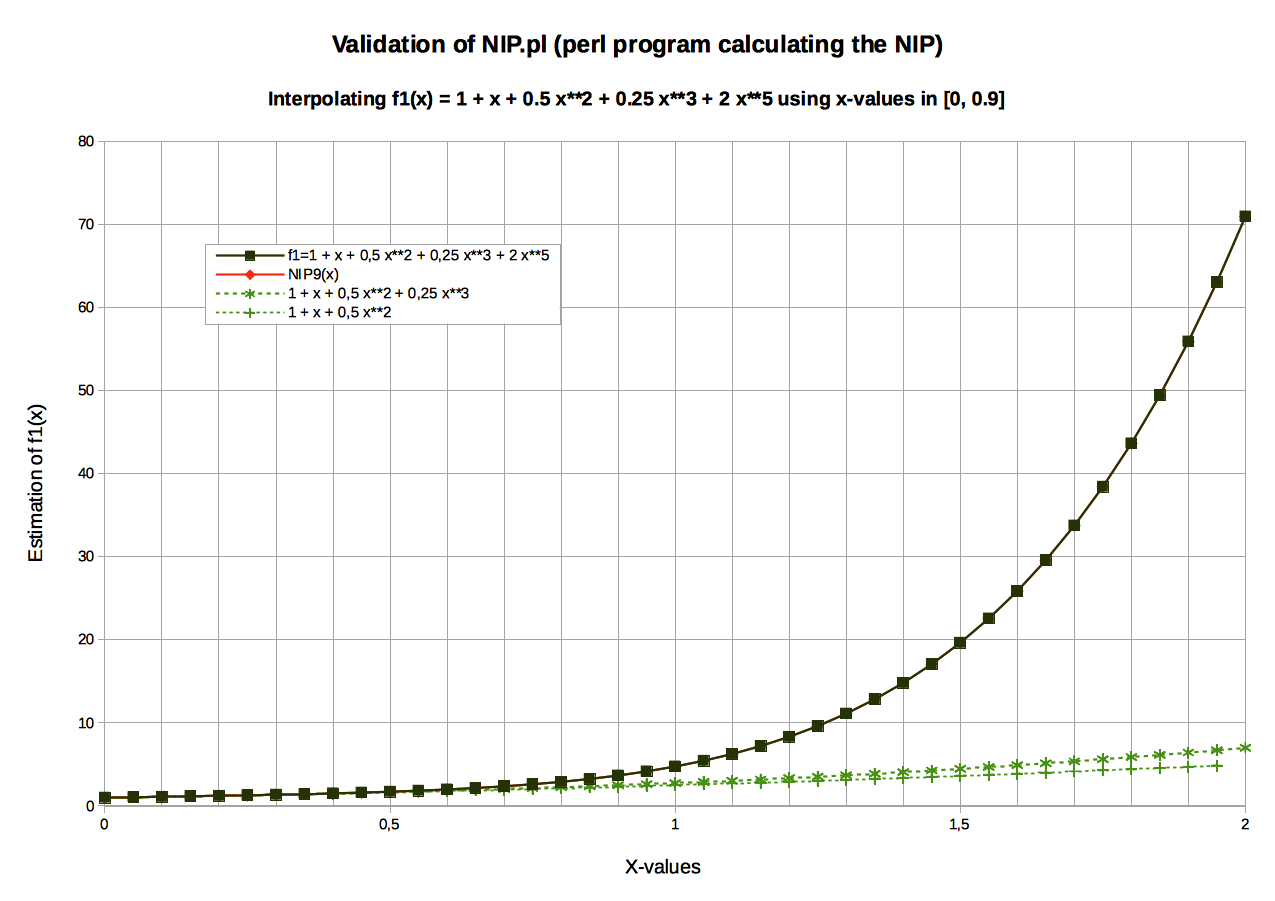
Graphic: NIP of polynomial f1(x)=1+ x+ 0.5 x2+ 0.25 x3+ 2 x5Input data (see NIP_input_StudyCase_1_Polynomial.txt)
- 10 (Xi,Yi)-values were used to calculate the NIP, N9(x): X0=0.00 to X9=0.9, Delta-X=0.10.
-
41 values were recalculated: X0=0.00 to X40=2.0,
Delta-X=0.05.
Rem: Some y-values have been interpolated (for x ≤ 0.9), others extrapolated (for 0.9 < x ≤ 2.0).
Results (see NIP_output_StudyCase_1_Polynomial.txt)
- All N9(Xi) fit exactly the original f(Xi): According to calc all differences equal to zero. The same result applies actually to N5.
-
ci coefficients of N5 and N9
Table: Comparison of the ci-coefficients for N5(x) and N9(x)Index of ci N5(x) N9(x) 0 +1.0000000000 +1.0000000000 1 +1.0000000000 +1.0000000000 2 +0.5000000000 +0.5000000000 3 +0.2500000000 +0.2500000000 4 +0.0000000000 +0.0000000000 5 +2.0000000000 +1.9999999999 6 +0.0000000002 7 -0.0000000002 8 +0.0000000001 9 -0.0000000000 In this particular case, where f1(x) is a polynomial, both NIP N5, N9 should ideally produce exactly the same result - which is the original set of all ci-coefficients in f1. Practically, N5(x) gives a better interpolation. The slight degradation is due to numerical imprecision (The values of coefficients c6 to c9 in N9 are obviously numerical noise).
-
Study Case: interpolate ex
f2(x)= ex, examined for x ∈ [0,4], (xi+1-xi)= Delta_x= 0.4perl NIP.pl -if NIP_input_StudyCase_2_exp_B.txt -of NIP_output_StudyCase_2_exp_B.txt (-mf NIP_message_StudyCase_2_exp_B.txt)
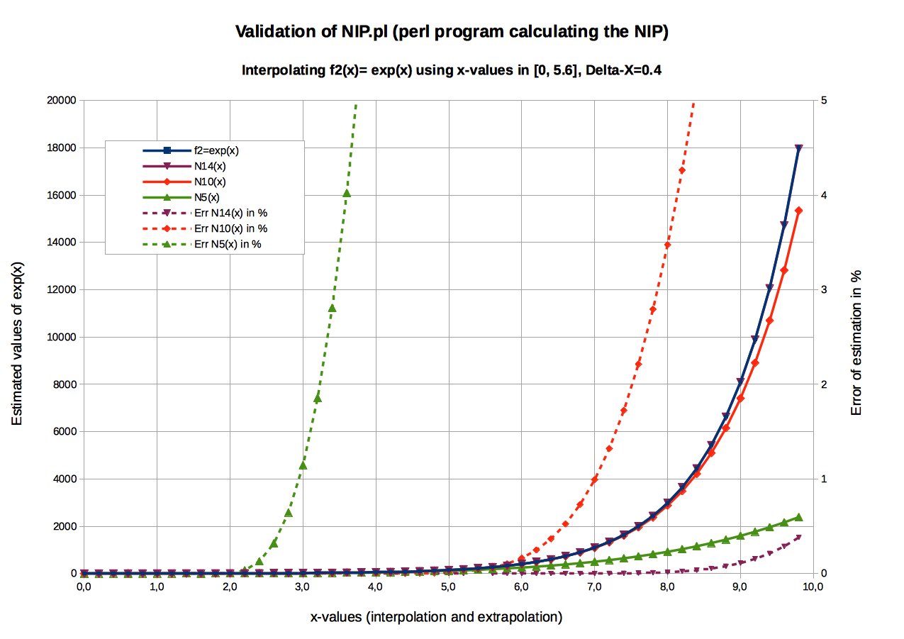
Graphic: NIP of polynomial f2(x) =exInput data (see NIP_input_StudyCase_2_exp_B.txt)
- 15 (Xi,Yi)-values were used to calculate N14(x): X0=0.00 to X10=5.6, Delta-X=0.40.
-
50 values were recalculated: X0=0.00 to X49=9.8,
Delta-X=0.20.
Rem: Some y-values have been interpolated (for x ≤ 5.6), others extrapolated (for 5.6 < x≤ 9.8).
Results (see NIP_output_StudyCase_2_exp_B.txt)
N14 produces good results over the whole recalculation range [0-9.8] (Its interpolation range is [0-5.6]).
N10 produces good results within a range [0-7.0] (Its interpolation range is [0-4.0]).
N5 produces good results within a range [0-2.8] (Its interpolation range is [0-2.0]).-
ci coefficients of N5, N10, N14 and T[ex]
Table: Convergence of the ci-coefficients toward the Taylor series T[ex]Index of ci N5 N11 N14 Taylor series T[ex] 0 +1.0000000000 +1.000000000 +1.0000000000 +1 1 +1.0041565261 +0.9999361463 +0.9999973245 +1 2 +0.4768052674 +0.5004629399 +0.5000216050 +0.5 3 +0.2123995333 +0.1652975971 +0.1665925953 +0.1666666667 4 +0.0015571296 +0.0438795661 +0.0418118925 +0.0416666667 5 +0.0234191137 +0.0061452376 +0.0081494533 +0.0083333333 6 +0.0027799887 +0.0015491374 +0.0013888889 7 -0.0003780932 +0.0000987721 +0.0001984127 8 +0.0001776319 +0.0000698567 +0.0000248016 9 -0.0000214749 -0.0000121544 +0.0000027557 10 +0.0000021764 +0.0000038663 +0.0000002756 11 -0.0000005916 +0.0000000251 12 +0.0000000744 +0.0000000021 13 -0.0000000051 +0.0000000002 14 +0.0000000002 +0.0000000000 The Taylor series T[ex)]= ∑n=0,∞ (xn/n!) is the limit to which Nk should converge, when k→∞.
The table above shows roughly how the ci-coefficients of NK converge toward the Taylor series, as K increases.
Beware: For i ≥ 13, the ci values cannot be clearly distinguished from the numerical noise (≈10-10) anymore!The graphic below shows the errors in the ci estimation of the ci coefficients for N5, N10 and N14.
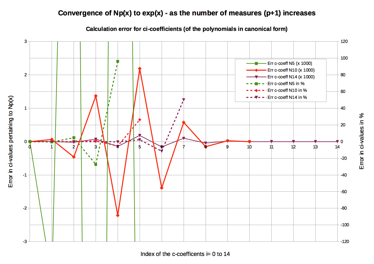
Graphic: Errors in the estimation of the ci-coefficients of selected NIPFor coefficients c1 to c7 there is a clear progression N5 > N10 > N14 > T[ex]. However, as the ci index increases (e.g. the ci value decreases), numerical imprecision gains influence. The relative errors in % shown on the secondary Y-axis may be an indicator of the phenomena: (absolute) values greater than 100% have been erased for the sake of readability.
-
Study Case: Interpolate sin(x)
f3(x)= sin(x), examined for x ∈ [0, 6.6], (xi+1-xi)= Delta_x= 0.6 (rem: 2.π ≈ 6.283)
perl NIP.pl -if NIP_input_StudyCase_3_sin.txt -of NIP_output_StudyCase_3_sin.txt (-mf NIP_message_StudyCase_3_sin.txt)
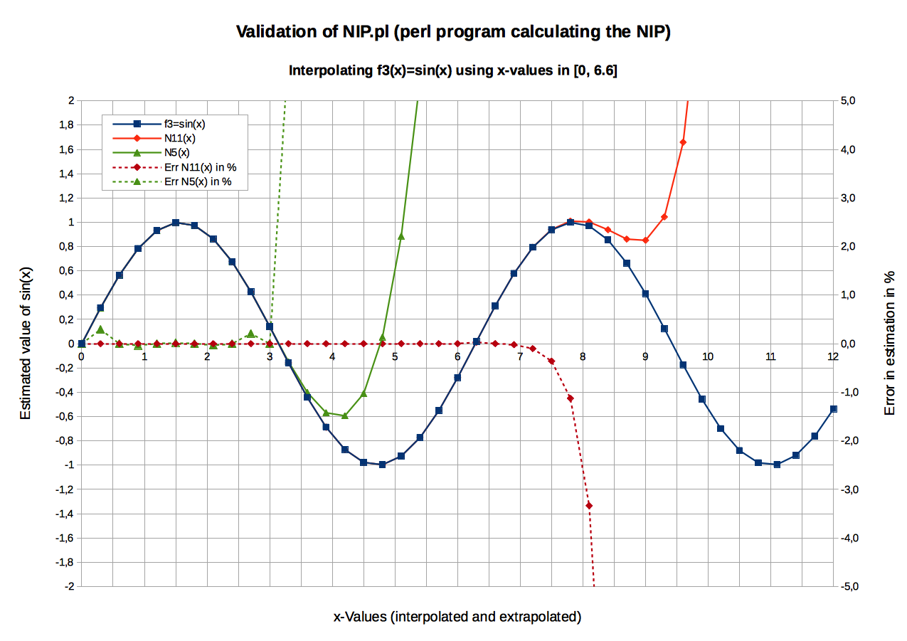
Graphic: NIP of f3(x)= sin(X)Input data (see NIP_input_StudyCase_3_sin.txt)
- 12 (Xi,Yi) values were used to calculate N11(x): X0=0.00 to X11=6.6, Delta-X=0.60.
-
42 values were recalculated: X0=0.00 to X41=12.3,
Delta-X=0.30.
Rem: Some y-values have been interpolated (for x ≤ 6.6), others extrapolated (for 6.6 < x ≤ 12.3).
Results (see NIP_output_StudyCase_3_sin.txt)
-
N11(x) produces good values within x-range [0, 7.80] (Its interpolation scope is [0, 6.60]).
N 5(x) produces good values within x-range [0, 3.00] - which corresponds to its interpolation scope. -
ci coefficients of N5, N11, and T[sin(x)]
Table: Convergence of the ci-coefficients toward the Taylor series T[sin(x)]Index of ci N5(x) N11(x) Taylor series T[sin(x)] 0 0.0000000000 0.0000000000 0 1 +0.9884512209 +1.0000246629 +1 2 +0.0431998861 -0.0001428261 0 3 -0.2237806822 -0.1663142431 -0.1666666667 4 +0.0332862131 -0.0004939005 0 5 +0.0005467594 +0.0087732791 +0.0083333333 6 -0.0002630934 0 7 -0.0000900869 -0.0001984127 8 -0.0000308189 0 9 +0.0000086901 +0.0000027557 10 -0.0000007253 0 11 +0.0000000210 -0.0000000251 The Taylor series T[sin(x)]=∑n=0,∞ (-1)n / (2n+1)! (x2n+1) is the limit to which Nk should converge, when k→∞.
The table above shows roughly how the ci-coefficients of NK converge, as K increases.
Note: All ci-coefficient values can still be clearly distinguished from the numerical noise but a few more coefficients will break the limit.- The graphic below shows the estimation errors for all ci in N5 and N11.
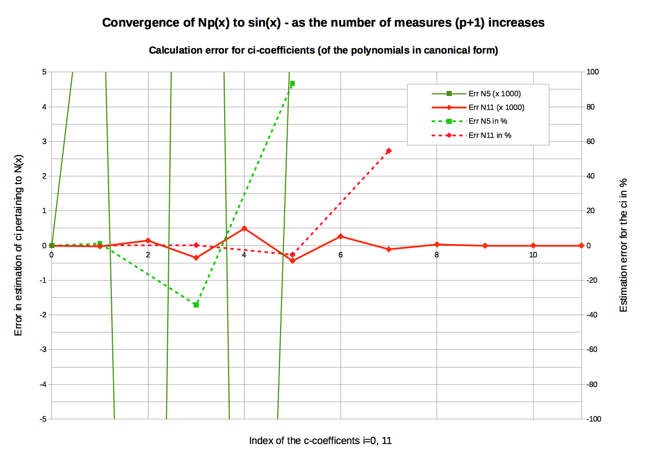
Graphic: Estimation errors for the ci-coefficients of NIP applied to sin(x)For coefficients c1 to c7 there is a clear improvement from N5 to N11 toward T[sin(x)]. As the ci index increases (e.g. the ci value decreases), the relative errors in % shown on the secondary Y-axis oscillates wilder and wilder. For the sake of readability, (absolute) values greater than 100% have been erased .
-
Study Case: Interpolate sqrt(1+x)
f4_1(x)= sqrt(x+1), calculated for x∈[0,2] and (xi+1-xi)=Delta_x=0.2
perl NIP.pl -if NIP_input_StudyCase_4_sqrt_1.txt -of NIP_output_StudyCase_4_sqrt_1.txt (-mf NIP_message_StudyCase_4_sqrt_1.txt)
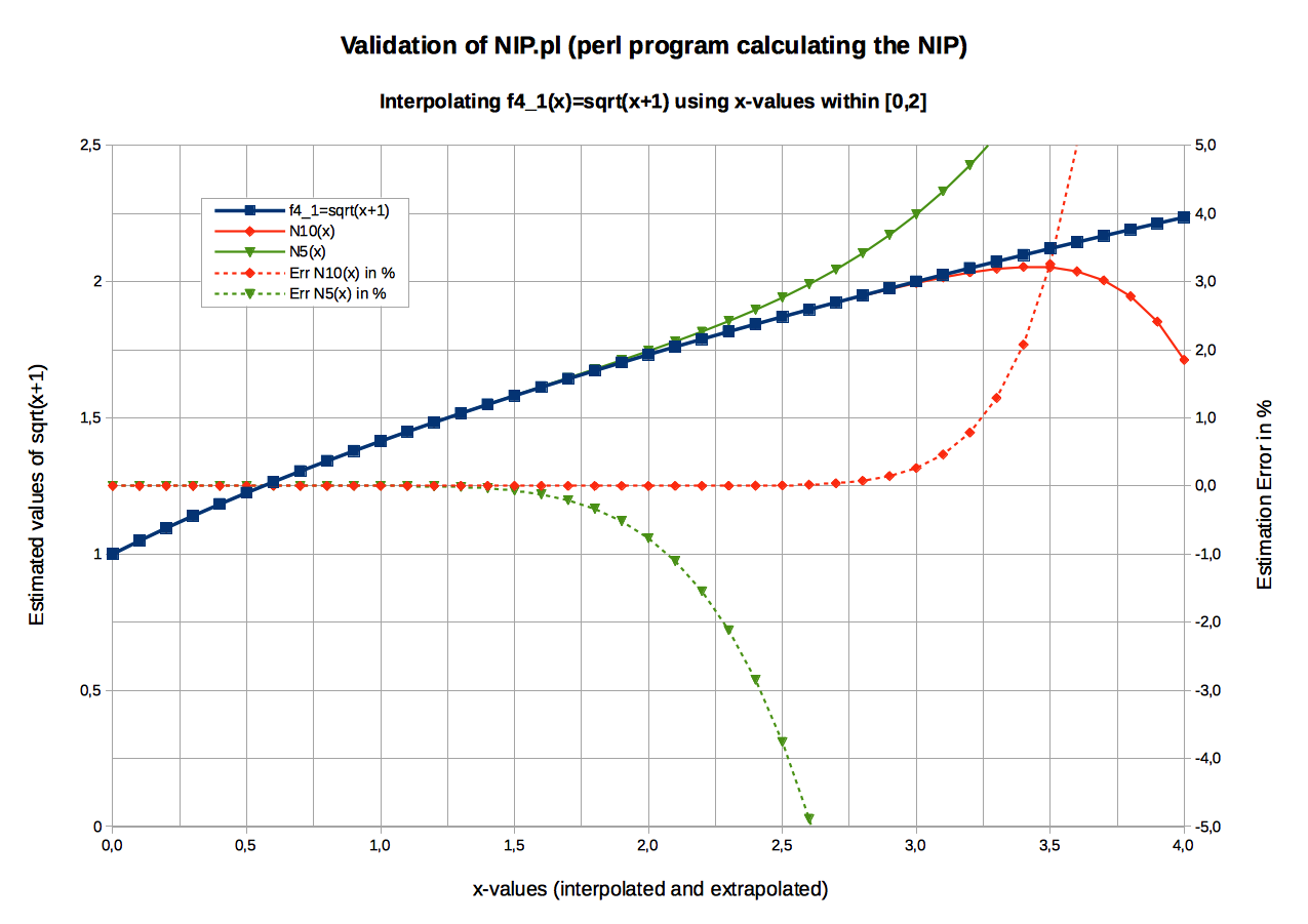
Graphic: NIP of f4_1(x)= sqrt(x+1)Input data (see NIP_input_StudyCase_4_sqrt_1.txt)
- 11 (Xi,Yi) values were used to calculate N10(x): X0=0.00 to X10=2.0, Delta-X=0.20.
-
42 values were recalculated: X0=0.00 to X41=4.1,
Delta-X=0.10.
Rem: Some y-values have been interpolated (for x ≤2.0), others extrapolated (for 2.0 < x ≤4.1).
Results (see NIP_output_StudyCase_4_sqrt_1.txt)
-
N10(x) produces good values within x-range [0, 3.3] (Its interpolation scope is [0, 2.0]).
N 5(x) produces good values within x-range [0, 2.1] (Its interpolation scope is [0, 1.0]). -
ci coefficients of N5, N10, and T[sqrt(x+1)]
Table: Convergence of the ci-coefficients toward the Taylor series T[sqrt(x+1)]Index of ci N5(x) N10(x) Taylor series T[sqrt(x+1)] 0 +1.0000000000 +1.0000000000 +1 1 +0.4998720084 +0.4999941272 +0.5 2 -0.1234444216 -0.1249091931 -0.125 3 +0.0553503036 +0.0619097542 +0.0625 4 -0.0224153672 -0.0368784515 -0.0390625 5 +0.0048510391 +0.0220985976 +0.02734375 6 -0.0116379230 -0.0205078125 7 +0.0048049210 +0.0161132813 8 -0.0013969429 -0.013092041 9 +0.0002488773 +0.0109100342 10 -0.0000202043 -0.0092735291 The Taylor series T[sqrt(1+x)]= ∑n=0,∞(0.5(0.5-1)...(0.5-n+1)/n!) xn is the limit to which Nk should converge, when k→∞.
The table above shows roughly how the ci-coefficients of NK converge, as K increases.
Note: In contrast to the situation in previous examples - ex, sin(x) - all ci-coefficient values are widely above the numerical noise: the interpolation potential is not yet exhausted.- The graphic below shows the estimation errors for all ci in N5 and N11.
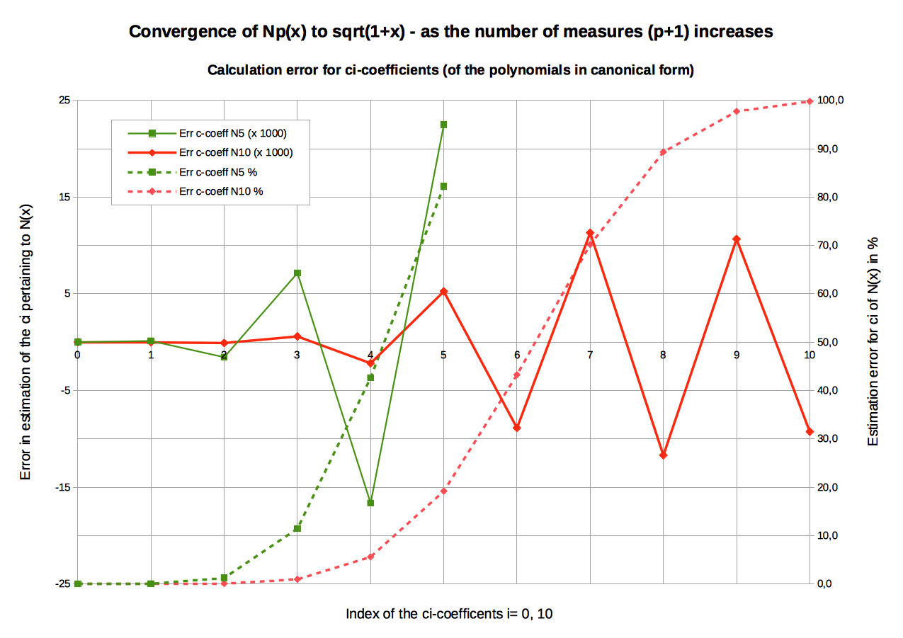
Graphic: Estimation errors for the ci-coefficients of NIP applied to sqrt(x+1)The graphic confirms the conclusions drawn before from the table: The Np suite converges smoothly toward T[sqrt(x+1)]. Increasing the number of measurement points used for calculating the NIP will certainly improve the precision of the results.
-
Study Case: Interpolate sqrt(x)
f4_2(x)= sqrt(x), calculated for x∈[0,2] and (xi+1-xi)=Delta_x=0.2
perl NIP.pl -if NIP_input_StudyCase_4_sqrt_2.txt -of NIP_output_StudyCase_4_sqrt_2.txt (-mf NIP_message_StudyCase_4_sqrt_2.txt)
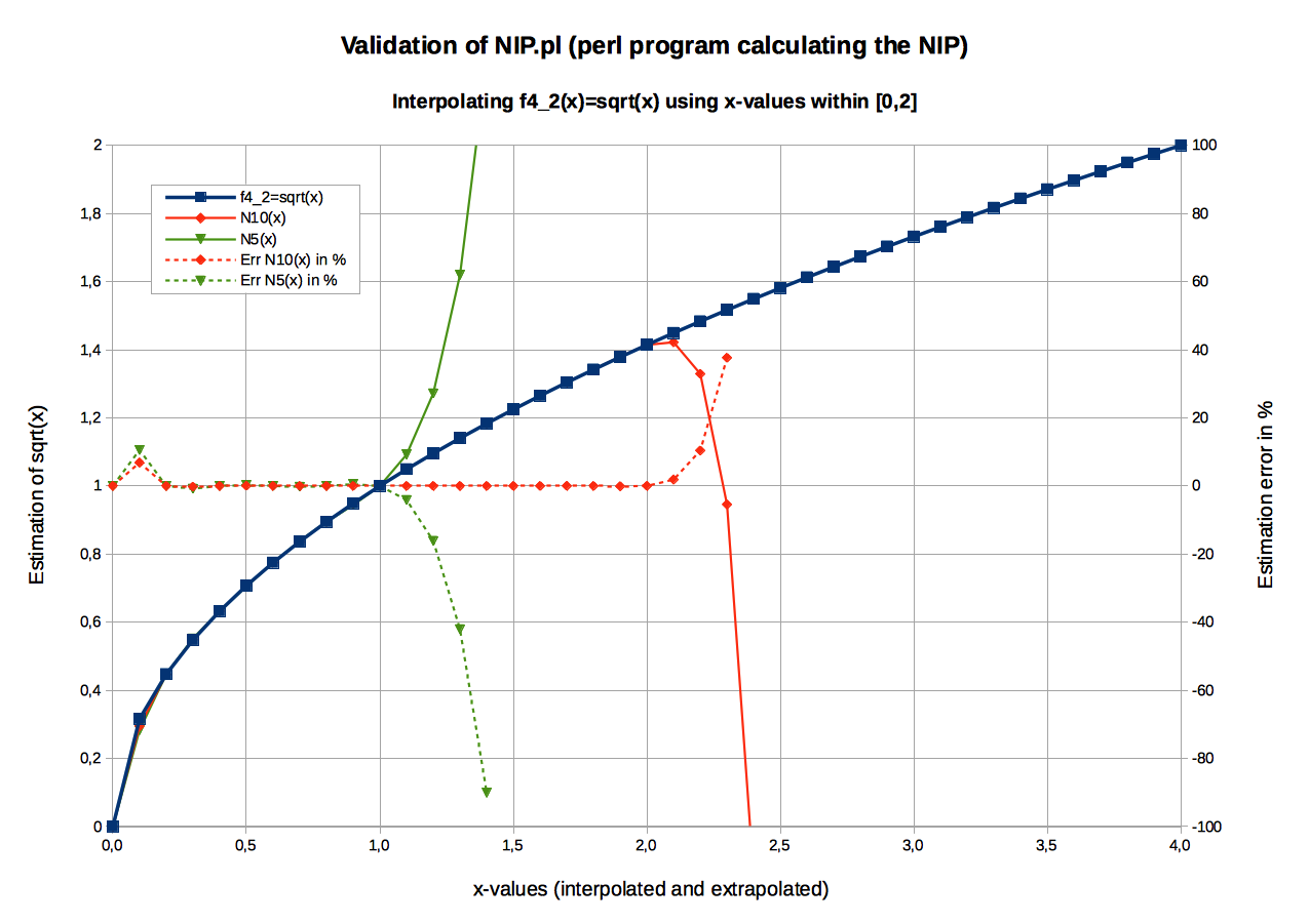
Graphic: NIP of f4_2(x)= sqrt(x)Input data (see NIP_input_StudyCase_4_sqrt_2.txt)
- 11 (Xi,Yi) values were used to calculate N10(x): X0=0.00 to X10=2.0, Delta-X=0.20.
-
42 values were recalculated: X0=0.00 to X41=4.1,
Delta-X=0.10.
Rem: Some y-values have been interpolated (for x ≤2.0), others extrapolated (for 2.0 < x ≤4.1).
Results (see NIP_output_StudyCase_4_sqrt_2.txt)
-
N10(x) produces good values within x-range [0, 2.0] (Its interpolation scope is [0, 2.0]).
N 5(x) produces good values within x-range [0, 1.0] (Its interpolation scope is [0, 1.0]).
Outside the interpolation range, the estimation error exceeds almost immediately the 100% limit: In order to preserve the readability of the graphical representation, the doted curves showing errors in % (linked to the secondary Y-axis) have been additionally truncated.
Also interesting to notice is the deviation pick occurring systematically at the first x value interpolated (x=0.1). -
ci coefficients of N5, N10
Table: Comparison of the ci-coefficients for N5(x) and N10(x)Index of ci N5(x) N10(x) 0 +0.0000000000 +0.0000000000 1 +3.6887261304 +4.2280735342 2 -10.2108662533 -17.0372885063 3 +17.5071419536 +50.8437458399 4 -14.8116527292 -98.8271330060 5 +4.8266508984 +127.3064766291 6 -109.6564207910 7 +62.4351224588 8 -22.5408190453 9 +4.6711946380 10 -0.4229517514 There is no Taylor series available for sqrt(x) in [0, 2], since its derivation values tend to +∞ as x tends to 0. In other words, there is no a priori convergence of the NK suite, when K grows.
Table and graphic show that ci values swing up and down. Presumably - and in contrast to all previous cases - this swinging effect will amplify as the number of measurements points used to calculate N(x) will increase (to be cleared).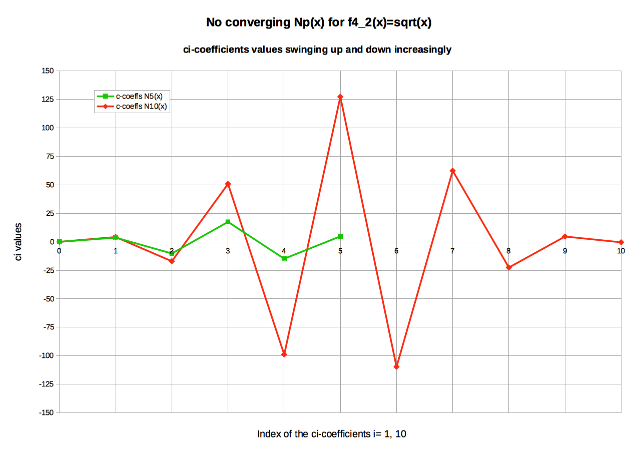
Graphic: Estimation of the ci-coefficients of NIP applied to sqrt(x) - Conclusions
Both functions f4_1(x)=sqrt(1+x) and f4_2(x)=sqrt(x) are similar: An affine transformation on the x values transposes the one function into the other. Notwithstanding their NIP resolution behaves quite differently:
- For f4_1(x)=sqrt(1+x), it shows a very good response.
- For f4_2(x)=sqrt(x), it shows a latent propensity toward instability.
The difficulty is due to the fact that f4_2(x)=sqrt(x) is not derivable at zero - i.e. no polynomial can correctly reproduce its curve near x=0.
-
Study Case: General conclusions
Program NIP.pl can correctly estimate the Newton Interpolation Polynomial N(x) for a given set of P+1 measures (Xi,Yi), i=0,P.
It will give acceptable results, if the measured values treated can - a priori - fit into the polynomial field i.e. if the unknown function f(x) to interpolate is analytic within the observed range.
- If the set of input values is extracted from a polynomial, NIP.pl will retrieve the polynomial in question.
- More generally, the NK suite will converge to the Taylor series T[f(x)], when K (i.e. the number of measures considered) increases.
The number of input points that can be handled (i.e. the highest degree of N(x) that can be calculated adequately) is limited by the numerical precision available. Most probably, NIP.pl can retrieve up to 15 coefficients.
The study cases focused so far on the adequate use of NIP. In cases where measurement points manifest ragged chaotic patterns, alternative methods are more appropriate e.g.
Fourier series.
Notwithstanding, it would be fun - and from the theoretical point of view just as rewarding - to analyze NIP solutions for input sets that clearly violate the required conditions of use. In order to study such cases in depth, it is proposed to provide NIP.pl with the ability to tackle heterogeneous sets - see chapter Further developments.
Following links may help increase one's understanding on the subject.
Web sites:
1 Mathews J. H. Lecture on Numerical Methods English 2 Chandra P. et all. Lecture on Numerical Methods English 3 Wikipedia Polynominterpolation (German, English) 4 FH Kärnten Informatikprojekt Newton Interpolationsformel German Download pdfs:
1 Shestopalov Y. Lecture on Interpolation Methods English Please beware: The above documentation results from a quick search: It can almost be considered a random output. In other words, a thorough investigation may have produced a different list.
Books (that I read on the subject):
1 Piskounov Calcul différentiel et intégral Tome 1 p266-268 Translation into French of the Russian original 2 Engeln-Müllges G., Reutter F. Numerische Mathematik für Ingenieure German -
Used perl sources and all discussed results are available for download in ZIP_Archive_NIP_1 from project reference Project_NIP_1.
ZIP_Archive_NIP_1 contains following files:
Table: List of contents from project NIP_1 available for downloadNIP.pl,NIP_lib.pm
perl sources: main program and library
NIP_input.txt
An example of input file, according to the default syntax.
\Study_Cases\ Sub-folder including all input and output files mentioned in the study cases.
NIP_StudyCases.ods (LibreOffice calc) has also been included: It includes input and output data of all study cases, as well as their analysis (especially the graphical output).Feel free to retrace every step by yourself.
Table: Brief history of versionsVersion date Description 0.0
May 2015
First version available for download:
- Calculates the Newton interpolation polynomial from a set of points (Xi, Yi)
- Reads Xi: X0, Delta-X= (Xi+1-Xi). For each Xi: Yi.
- Reads a set of recalculation points whose Xi are defined similarly to the input X values.
0.1 June 2015
Following extensions have been implemented:
- Each NIP selected for recalculation/validation will be automatically transposed into canonical form (Estimation of the ci-coefficients out of the bi-coefficients).
Rem: At any given time, only one version will be available for download: the last published update.
-
I do not expect any portability issues:
- I developed NIP.pl on OSX Yosemite version 10.10.3 using perl version v5.18.2.
- I successfully run NIP.pl, as is, on microsoft windows 7 Ultimate, Service Pack 1 using Strawberry perl (64-bit) version v5.20.2.1.
If someone gets into trouble, please send a message to Feedback explaining the circumstances. I will update this document accordingly.
-
Here a few ideas to implement in further versions of NIP.pl in order of preference.
-
Read heterogeneous measurement sets :
Free defined (non equidistant) Xi sets open new possibilities of studying NIP: What happens, if the Xi set is not monotone, if areas are more densely measured than others, etc. Programing hint: Only a few lines of code need to be modified (reading section INPUT_DATA). -
Introduce normalized intervals:
All Xi values shall be projected into an given interval before treatment e.g. [0,1], [1,2]. In my opinion, this transformation should work like some sort of data conditioning (to be cleared). Programing hint: In this case, one function - performing an (affine) transformation - must be coded. -
Advanced resolution of the linear equations system:
A radical modification is to resolve the NIP linear equations system (lower triangular) with algorithms that ensure that all bi are estimated with the same precision (unlike the current implementation). Beware: A great deal of preliminary coding is required - or a good mathematical library (Does anybody know about perl libs for matrices manipulation?) .
-